5. PyTorch Models
Interfacing with PyTorch allows us to conveniently fit neural network potentials using descriptors that exist in LAMMPS. We may then use these neural network models to run high-performance MD simulations in LAMMPS. When fitting atom-centered neural network potentials, we incorporate a general and performant approach that allows any descriptor as input to the network. This is achieved by pre-calculating descriptors in LAMMPS which are then fed into the network, as shown below.
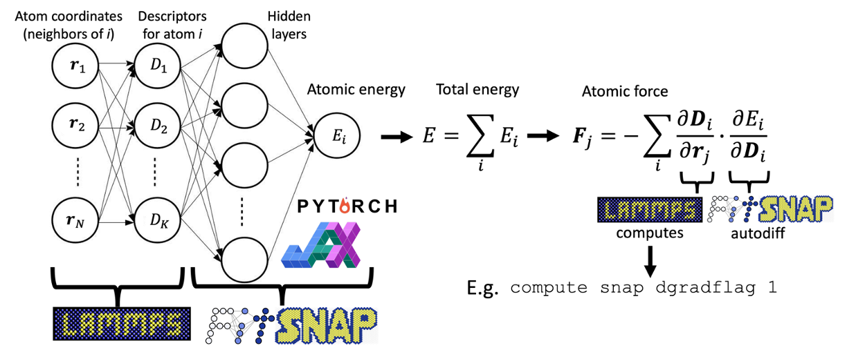
To calculate forces, we use the general chain rule expression above, where the descriptor derivatives are analytically extracted from LAMMPS. These capabilities are further explained below.
5.1. Fitting Neural Network Potentials
Similarly to how we fit linear models, we can input descriptors into nonlinear models such as
neural networks. To do this, we can use the same FitSNAP input script that we use for linear
models, with some slight changes to the sections. First we must add a PYTORCH section,
which for the tantalum example looks like:
[PYTORCH]
layer_sizes =  num_desc 60 60 1
learning_rate = 1.5e-4
num_epochs = 100
batch_size = 4
save_state_output = Ta_Pytorch.pt
energy_weight = 1e-2
force_weight = 1.0
training_fraction = 1.0
multi_element_option = 1
We must also add a nonlinear = 1 key in the CALCULATOR section, and set
solver = PYTORCH in the SOLVER section. Now the input script is ready to fit a
neural network potential.
The PYTORCH section keys are explained in more detail below.
layer_sizesdetermines the network architecture. We lead with anum_descparameter which tells FitSNAP that the number of nodes in the first layer are equal to the number of descriptors. The argument here is a list where each element determines the number of nodes in each layer.learning_ratedetermines how fast the network minimizes the loss function. We find that a learning rate around1e-4works well when fitting to forces, and when using our current loss function.num_epochssets the number of gradient descent iterations.batch_sizedetermines how many configs to average gradients for when looping over batches in a single epoch. We find that a batch size around 4 works well for our models.save_state_outputis the name of the PyTorch model file to write after every epoch. This model can be loaded for testing purposes later.save_state_inputis the name of a PyTorch model that may be loaded for the purpose of restarting an existing fit, or for calculating test errors.energy_weightis a scalar constant multiplied by the mean squared energy error in the loss function. Declaring this parameter will override the weights in the GROUPS section for all configs. We therefore call this the global energy weight. If you want to specify energy weights for each group, do so in the GROUPS section.force_weightis a scalar constant multiplied by the mean squared force error in the loss function. Declaring this parameter will override the weights in the GROUPS section for all configs. We therefore call this the global force weight. If you want to specify force weights for each group, do so in the GROUPS section.training_fractionis a decimal fraction of how much of the total data should be trained on. The leftover1.0 - training_fractionportion is used for calculating validation errors during a fit. Declaring this parameter will override the training/testing fractions in the GROUPS section for all configs. We therefore call this the global training fraction. If you want to specify training/testing fractions for each group, do so in the GROUPS section.multi_element_optionis a scalar that determines how to handle multiple element types.1: All element types share the same network. Descriptors may still be different per type.
2: Each element type has its own network.
3: (Coming soon) One-hot encoding of element types, where each type shares the same network.
manual_seed_flagset to 0 by default, can set to 1 if want to force a random seed which is useful for debugging purposes.shuffle_flagset to 1 by default, determines whether to shuffle the training data every epoch.
5.2. Loss Function
When fitting neural network potentials we minimize the sum of weighted energy and force mean squared errors:
where
\(M\) is the number of configurations in the training set.
\(m\) indexes a particular configuration.
\(N_m\) is the number of atoms for configuration \(m\)
\(w_m^E\) is the energy weight of configuration \(m\). These weights can be set by designating the particular weights in the [GROUPS] section, or by declaring a global weight in the
[PYTORCH]section, which will override the group weights.\(\theta\) represents all the model fitting parameters (e.g. the trainable coefficients in a neural network).
\(\hat{E}_m(\theta)\) is the model predicted energy of configuration \(m\)
\(E_m\) is the target ab initio energy of configuration \(m\), subtracted by the LAMMPS reference potential declared in the [REFERENCE] section.
\(i\) indexes a Cartesian index of a single atom; we lump Cartesian indices and atom indices into a single index here.
\(w_m^F\) is the force weight of configuration \(m\). These weights can be set by designating the particular weights in the [GROUPS] section, or by declaring a global weight in the
[PYTORCH]section, which will override the group weights.\(\hat{F}_{mi}(\theta)\) is a model predicted force component \(i\) in configuration \(m\)
\(F_{mi}\) is a target ab initio force component \(i\) in configuration \(m\), subtracted by the LAMMPS reference potential force declared in the [REFERENCE] section.
This loss also gets evaluated for the validation set for each epoch, so that the screen output looks something like:
----- epoch: 0
Batch averaged train/val loss: 4.002996124327183 4.072216800280979
Epoch time 0.3022959232330322
----- epoch: 1
Batch averaged train/val loss: 2.3298445120453835 1.1800143867731094
Epoch time 0.2888479232788086
----- epoch: 2
Batch averaged train/val loss: 0.6962545616552234 0.8775447851845196
Epoch time 0.26888108253479004
----- epoch: 3
Batch averaged train/val loss: 0.3671231440966949 0.6234593641545091
Epoch time 0.26917600631713867
The first column is the weighted training set loss function, and the second column is the weighted validation set loss function (which is not included in fitting). While the loss function units themselves might not be meaningful for error analysis, we output model predictions and targets for energies and forces in separate files after the fit, as explained below.
5.3. Outputs and Error Calculation
Unlike linear models, PyTorch models do not output statistics in a dataframe. Instead we output energy and force comparisons in separate files, along with PyTorch models that can be used to restart a fit or even run MD simulations in LAMMPS.
5.3.1. Error/Comparison files
After training a potential, FitSNAP produces outputs that can be used to intrepret the quality of a
fit on the training and/or validation data. Basic error metrics for the total set and groups are
output in the metric file declared in the [OUTFILE] section:
[OUTFILE]
metrics = Ta_metrics.dat # filename for Ta example
In this example, we write error metrics to a Ta_metrics.dat file.
The first line of this file describes what the columns are:
Group  Train/Test   Property   Count   MAE    RMSE
...
where Count is the number of configurations used for energy error, or atoms used for force error.
Fitting progress may be tracked in the loss_vs_epochs.dat file, which tracks training and validation losses.
More detailed fitting metrics are obtained if the following flags are declared true in the
[EXTRAS] section:
[EXTRAS]
dump_peratom = 1   # write per-atom fitting metrics
dump_perconfig = 1 # write per-config fitting metrics
dump_configs = 1   # write a pickled list of Configuration objects
The following comparison files are written after a fit:
peratom.dat: Fitting information for each atom, such as truth and predicted forces.
The first line of this file describes what the columns are:
Filename Group AtomID Type Fx_Truth Fy_Truth Fz_Truth Fx_Pred Fy_Pred Fz_Pred Testing_Bool
perconfig.dat: Fitting information for each configuration, such as truth and predicted energies.
The first line of this file describes what the columns are:
Filename Group Natoms Energy_Truth Energy_Pred Testing_Bool
configs.pickle: Structural, descriptor, and fitting info for each configuration.
This is a pickled list of Configuration objects. Each item in the list contains all associated information of a configuration.
5.3.2. PyTorch model files
FitSNAP outputs two PyTorch .pt models file after fitting. One is used for restarting a fit
based on an existing model, specifically the model name supplied by the user in the
save_state_output keyword of the input script. In the Ta_PyTorch_NN example
we can see this keyword is Ta_Pytorch.pt. This file will therefore be saved every epoch, and
it may be fed into FitSNAP via the save_state_input keyword to restart another fit from that
particular model.
The other PyTorch model is used for running MD simulations in LAMMPS after a fit. This file has the
name FitTorch_Pytorch.pt, and is used to run MD in LAMMPS via the ML-IAP package. An example
is given for tantalum here: https://github.com/FitSNAP/FitSNAP/tree/master/examples/Ta_PyTorch_NN/MD
5.3.3. Calculate errors on a test set
Users may want to use models to calculate errors on a test set that was completely separate from the training/validation sets used in fitting. To do this, we change the input script to read an existing PyTorch model file, e.g. for Ta:
[PYTORCH]
layer_sizes =  num_desc 60 60 1
learning_rate = 1.5e-4
num_epochs = 1 ##### Set to 1 for calculating test errors
batch_size = 4
save_state_input = Ta_Pytorch.pt ##### Load an existing model
energy_weight = 1e-2
force_weight = 1.0
training_fraction = 1.0
multi_element_option = 1
num_elements = 1
Notice how we are now using save_state_input instead of save_state_output, and that
we set num_epochs = 1. This will load the existing PyTorch model, and perform a single epoch
which involves calculating the energy and force comparisons (mentioned above) for the current model,
on whatever user-defined groups of configs in the groups section.We can therefore use the energy and
force comparison files here to calculate mean absolute errors, e.g. with the script in
the Ta_PyTorch_NN example
5.4. Training Performance
As seen in the Ta_Pytorch_NN example, fitting to ~300 configs (each with ~12 atoms) takes
about ~0.2 s/epoch. The number of epochs required, and therefore total time of your fit, will depend
on the size of your dataset and the batch_size. For example, the Ta_Pytorch_NN example
might take ~200 epochs to fully converge (see loss_vs_epochs.dat). In this example, however,
we used batch_size=4, meaning that each epoch involved ~300/4 = ~75 gradient descent
minimizations as we cycled through batches. For much larger datasets, the network will experience
more cycles through the batches with each epoch, and therefore may require less epochs to reach
the same convergence.
For data sets of ~10,000 configs and ~50 atoms per config, training will take ~1 hour, or about 20 seconds per epoch. This can consume about ~20 GB of RAM.
Computational scaling is roughly O(num_atoms*num_neighs) where num_atoms is the
total number of atoms in the training set, and num_neighs is the average number of neighbors
per atom.
Mini-batch network training is embarassingly parallel up to the batch size, but currently FitSNAP does not support parallelized NN training.
5.4.1. GPU Acceleration
FitSNAP supports GPU acceleration via PyTorch. With small batch sizes, however, most of the benefit of GPU parallelization comes from evaluating the NN model and calculating gradients. You will not see a large benefit of GPUs using a small batch size unless you have a large NN model (e.g. > 1 million parameters). If you have a small model, you will see a speedup on GPUs using a large enough batch size.