4. Linear Models
FitSNAP can perform linear regression to obtain models of the form
where
\(s\) indexes a particular configuration of atoms
\(E_s\) is the potential energy of configuration \(s\)
\(i\) indexes a particular atom
\(N_s\) is the number of atoms in configuration \(s\)
\(\boldsymbol{\beta}_i\) is a vector of fitting coefficients for atom \(i\)
\(\boldsymbol{B}_i\) is a vector of atomic environment descriptors for atom \(i\)
The settings for SNAP descriptors are explained in the [BISPECTRUM] section.
For this linear regression problem we solve the following matrix problem as explained in Thompson et. al.
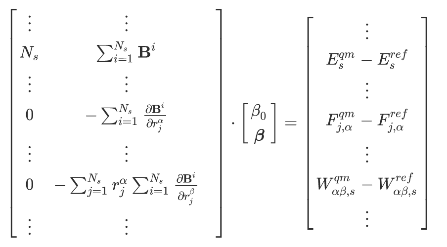
where
\(\frac{\boldsymbol{B}_i}{r_j^{\alpha}}\) is the gradient of descriptor \(\boldsymbol{B}_i\) with respect to \(r_j^{\alpha}\), the \(\alpha\) Cartesian direction of atom \(j\).
\(E^{qm}_s\) is the quantum mechanical target energy for configuration \(s\)
\(E^{ref}_s\) is the reference energy of a potential that is overlayed on the linear regression model, as declared in the [REFERENCE] section
\(F^{qm}_{j,\alpha}\) is the quantum mechanical target force for atom \(j\) in the \(\alpha\) direction.
\(F^{qm}_{j,\alpha}\) is the reference force for atom \(j\) in the \(\alpha\) direction, from a potential that is overlayed on the linear regression model, as declared in the [REFERENCE] section.
\(W_{\alpha \beta, s}\) is virial in the \(\alpha\) and \(\beta\) directions for configuration \(s\), where both quantum mechanical target and reference virials are included on the right-hand side of the matrix equation.
FitSNAP solves this matrix problem using SVD and supports other solvers as well. For more details on settings used for descriptors and solvers, please see the docs on FitSNAP Input Scripts.
4.1. Outputs
The outputs for linear models are explained here. For nonlinear models, please see the PyTorch models output section. After running a linear model fit, the following outputs will be produced:
FitSNAP.dfis a Pandas dataframe with rows corresponding to the linear fitting matrix as shown above. We have interactive examples of examining this dataframe and calculating detailed errors from it in our Colab Python notebook tutorial.*_metrics.mdis a markdown file containing mean absolute errors and RMSEs for your dataset. If using LAMMPS metal units, energy errors are in eV, and force errors are in eV/Angstrom. The prefix name of this file depends on themetricsparameter declared in the [OUTFILE] section.LAMMPS-ready potential files. For example if fitting with SNAP descriptors, this will create
*_pot.snapparamand*_pot.snapcoefffiles with prefix names depending on thepotentialparameter declared in the [OUTFILE] section. To use these files with LAMMPS, please refer to the LAMMPS documentation.
4.2. Uncertainty Quantification (UQ)
Linear models have uncertainty quantification (UQ) capabilitiies in the form of extra solvers, which
are explain here. UQ solvers output a covariance.npy file in addition to performing a fit.
We incorporate an analytical Bayesian UQ solver denoted by solver = ANL in the input script. This
is declared like:
solver = ANL
nsam = 133            #this is the number of sample fits requested to be drawn from the distribution
cov_nugget = 1.e-10   #this is the small number to be added to the matrix inverse for better conditioning
4.3. In development UQ solvers
In general we recommend the use of the ANL solver. The following UQ solvers, however, are
experimental and in development.
4.3.1. OPT
solver = OPT
The standard least-squares fit, but solving the optimization problem instead of SVD or matrix inversions. Can be useful when matrices are ill-conditioned, or when we add regularization.
4.3.2. MCMC
solver = MCMC
nsam = 133            #this is the number of sample fits requested to be drawn from the distribution
mcmc_num = 1000       #this is the number of total MCMC steps requested
mcmc_gamma = 0.01     #this is the MCMC proposal jump size (smaller gamma increases the acceptance rate)
MCMC sampling, currently assuming constant noise size, but unlike the ANL case, there is flexibility if one plays with the log-post function.
4.3.3. MERR
solver = MERR
nsam = 133                #this is the number of sample fits requested to be drawn from the distribution
merr_method = iid         #specific liklihood model: options are iid, independent identically distributed, and abc, approximate bayesian computation, and full (too heavy and degenerate, not intended to be used yet)
merr_mult = 0             #0 is additive model error, 1 is multiplicative
merr_cfs = 5 44 3 49 10 33 4 39 38 23       #can provide either a list of coefficient indices to embed on, or "all"
cov_nugget = 1.e-10       #this is the small number to be added to the matrix inverse for better conditioning
Model error embedding approach - powerful but very slow. Requires an optimization that does not run in parallel currently, and is not guaranteed to converge.
4.3.4. BCS
solver = BCS
Fitting with Bayesian compressive sensing, need to learn how to prune bispectrum bases in order for this to be useful. Not working properly yet.